Understanding the World with Data

Intro and Syllabus

Welcome to Stat 20! We are very excited to have you here this semester. There are no reading questions for today’s content, but make sure that you have:

• gotten the name of your instructor and in-class tutors
• read the syllabus and asked any questions you have about it on your lecture’s corresponding Ed thread
• taken a look at the first problem set.

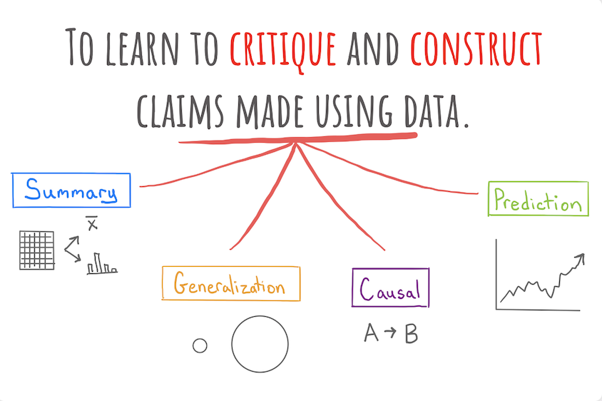
The goal of our course is to construct and critique claims made using data. This raises the question: what type of claims can be made? Four of the five units in this course will center around a specific type of claim (the other unit being probability.) We provide definitions for each of the claims below!

Types of Claims

Summary

A numerical, graphical, or verbal description of an aspect of data that is on hand.

Example: Using data from the Stat 20 class survey, the proportion of respondents to the survey who reported having no experience writing computer code is 70%.

Generalization

A numerical, graphical, or verbal description of a broader set of units than those on which data was been recorded.

Example: Using data from the Stat 20 class survey, the proportion of Berkeley students who have no experience writing computer code is 70%.

Causal Claim

A claim that changing the value of one variable will influence the value of another variable.

Example: Data from a randomized controlled experiment shows that taking a new antibiotic eliminates more than 99% of bacterial infections.

Prediction

A guess about the value of an unknown variable, based on other known variables.

Example: Based on reading the news and the price of Uber’s stock today, I predict that Uber’s stock price will go up 1.2% tomorrow.

Intro to R and RStudio

If our goal is to construct a claim with data, we need a tool to aid in the construction. Our tool must be able to do two things: it must be able to store the data and it must be able to perform computations on the data.

In high school, you gained experience with one such tool: the graphing calculator. This fits our needs: you can enter a list of number into a graphing calculator like the Ti-84, it can store that list and it can execute computations on it, such as taking its sum. But the types of data that a calculator can store are very limited, as is the volume of data, as are the options for computation.

In this class, we will use a tool that is far more powerful: the computer language called R. The Ti-84 is to R what a tricycle is to the space ship. One of these tools can bring you to the end of the block; the other to the moon.

R is one of the most powerful languages for doing statistics and data science. One of the reasons for its power and popularity is that it is both free and open-source. This turns languages like R into something that resembles Wikipedia: a collaborative effort that is constantly evolving. Extensions to the R language have been authored by professional programmers¹, people working in industry and government², professors³, and students like you⁴.

You’ll be writing and running code through an app called RStudio. Beyond writing R code, RStudio allows you to manage your files and author polished documents that weave together code and text. RStudio can be run through a browser and we have set up an account for you that you can access by sending a browser tab to https://stat20.datahub.berkeley.edu/ or clicking the link in the upper right corner of the course website.

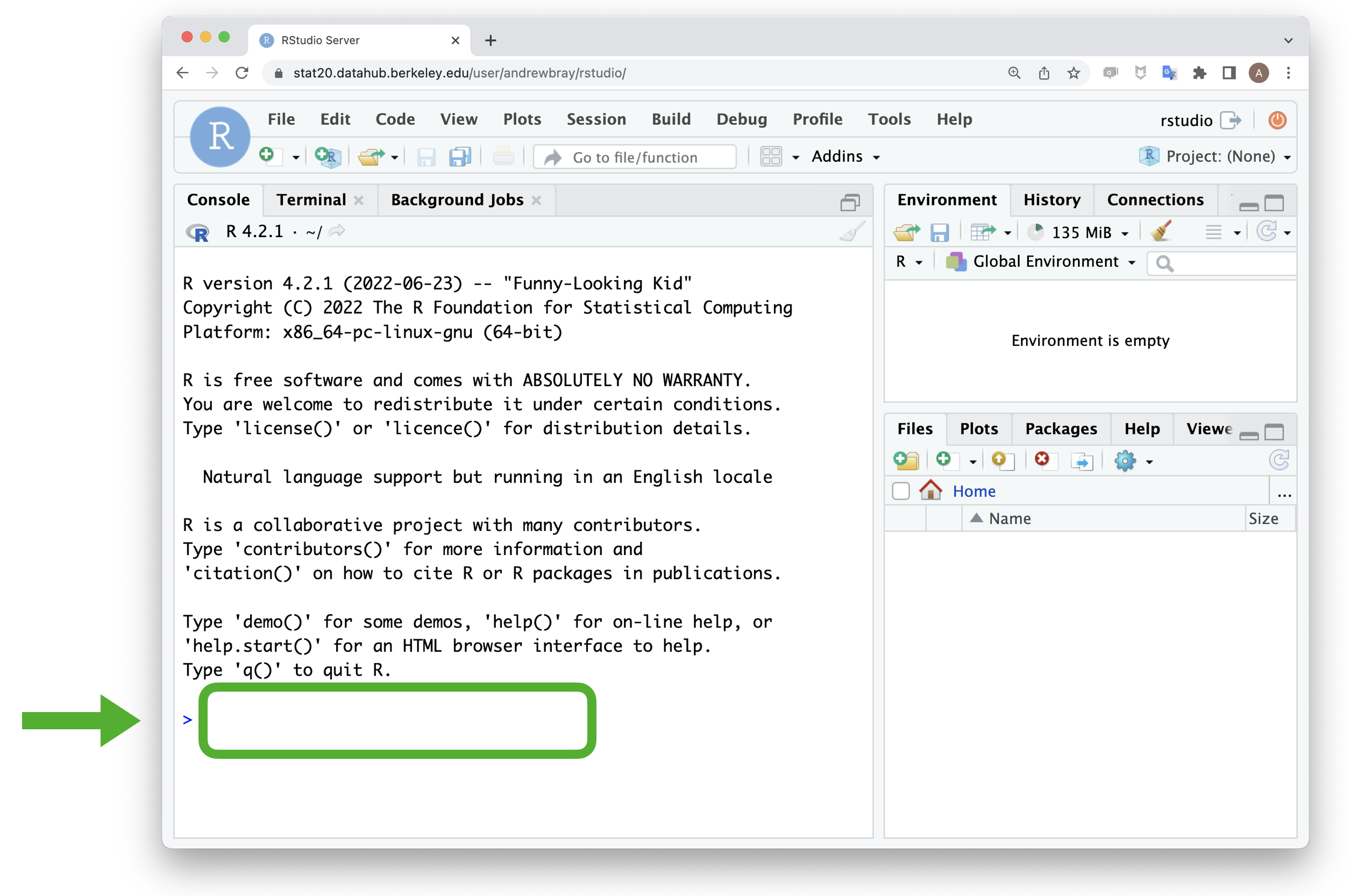
When you log into RStudio, the place where you can type and run R code is called the console and it’s located right here:

Figure 1: The R console in RStudio.

Code along

As you read through these notes, keep RStudio open in another window to code along at the console.

R as a Calculator

Although R is like a space ship capable of going to the moon, it’s also more than able to go to the end of the block. Type the sum 1 + 2 into the console (the area to the right of the >) and press Enter. What you should see is this:

1 + 2

[1] 3

All of the arithmetic operations work in R.

1 - 2

[1] -1

1 * 2

[1] 2

1 / 2

[1] 0.5

Each of these four lines of code is called a command and the response from R is the output. The [1] at the beginning of the output is there just to indicate that it is the first element of the output. This helps you keep track of things when the output spans many lines.

Although it is easiest to read code when the numbers are separated from the operator by a single space, it’s not necessary. R ignores all spaces when it runs your code, so each of the following also work.

1/2

[1] 0.5

1   /         2

[1] 0.5

You can add exponents by using ^, but don’t forget about the order of operations. If you want an alternative ordering, use parentheses.

2 ^ 3 + 1

[1] 9

2 ^ (3 + 1)

[1] 16

Footnotes

1. The googlesheets4 package, which reads spreadsheet data into R was authored by Jenny Bryan, a developer at Posit: :https://googlesheets4.tidyverse.org/.

2. The statistics office of the province of British Columbia maintains a public R package with all of their data: https://bcgov.github.io/bcdata/

3. Dr. Christopher Paciorek in the Department of Statistics at UC Berkeley maintains a package to fit a very broad class of statistical models called Bayesian Models: https://r-nimble.org/.

4. Simon Couch wrote the stacks package for model ensembling while an undergraduate https://stacks.tidymodels.org/index.html.